Purdue University 1997 Swine Day Report
D. DiPietre, L. Fuchs, and R. Tubbs
University of Missouri-Columbia; Senior Lending Officer, AgriBank, St. Paul, MN;
and Green River Swine Consultation, Bowling Green, KY
The first step in any knowledge-based evaluation of your operation is to understand your own system. Are you measuring production accurately? Are pigs accounted for accurately in each stage of production? Are all purchases and sales recorded and passed through farm record systems in a timely fashion? Do physical inventory counts reconcile with computer-generated numbers? How many "adjustments" and "unrecorded deaths" are necessary at the end of the month to reconcile records? Before making any judgments or comparisons, your own system needs to be as accurate as possible.
In the past, one of the main concerns of consultants, both independent and those employed by the extension service, was to convince producers of the necessity of keeping good records. Those days are over. Today, an accurate set of production and financial records is expected in order to make any kind of rational decision concerning a swine operation. The challenge for producers is to use the data that is available from record-keeping systems to make good decisions.
Before productivity can be analyzed, producers must understand their record-keeping system. Many producers use financial records exclusively to manage their income tax issues. This is like buying a sports car and never shifting it out of first gear. Production and financial records are perhaps the most under-utilized of all assets available to producers.
There are many record-keeping systems to assist producers in keeping accurate inventories and compiling historical data. The more useful systems are also diagnostically oriented. Record-keeping systems should use terms and standards commonly accepted in the industry. We recommend the adoption of the standardized production and financial system being completed by NPPC.
The ability to do production and cost analysis, benchmarking and establish production and financial control systems within the pork industry will improve immensely with the adoption of the production and financial standards and definitions being developed by NPPC. There are some general areas of concern that should be understood by any producer who wants to be effective at using records to improve his operation. The first is simply the accounting system used. Accrual accounting is necessary to really understand inventories, asset or inventory management, expense management, debt management and profits. Without accrual accounting, meaningful analysis is impossible.
Accrual financial statements, together with accurate production records, all recorded in a standard format, are the source for establishing understanding of your system, analyzing it over time and providing control to achieve your goals.
Although comparing one swine operation's productivity and financial performance with others is useful, it can be unreliable.
Common mistakes made in comparing production and financial efficiency and throughput measures from farm to farm are:
Being influenced by reports of extreme values in a variety of production parameters, including feed efficiency, building costs, pigs/sow/year, and costs of production, market price received, etc. If the value sounds too good to be true, it probably is. Many of these reports are for systems that are new, enjoying the "honeymoon" period, and do not represent long-term sustainable levels of achievement.
Comparing the performance of production systems that are too different to allow meaningful comparisons.
Comparing the performances of operations with record-keeping systems that are different or that calculate measures differently.
Making important decisions based on rumor or the latest "hot" issue affecting the industry. Producers must be able to separate fact from fiction and make decisions based on information relevant to their own operations.
A common problem that we observe with record-keeping software for production systems is that producers often create their own spreadsheet templates. The resulting program may be narrowly focused on the individual producer's pet concerns and may not address the issues that a consultant or lender believes are important. Often, these homemade programs report only historical data, without providing any diagnostic or problem-solving help on current problems. These programs usually limit the producer's ability to understand their system. Switching to a standardized record-keeping system will enhance your ability to conduct meaningful production and financial analyses.
To avoid invalid comparisons, you must understand the record-keeping system that is being used, when the data are recorded, the lag-time from when events occur to when data are entered into the records program, the data integrity level of the farm, and the processes that are followed to ensure accuracy of the data.
In order to achieve a competitive position and remain there, producers must implement a continual proactive process of improvement. One method is to identify the best practices of the industry. As these are identified, an evaluation process begins to determine if employing these practices within your own operation could result in increased profitability. If increased profits are likely, planning is undertaken, capital is sought, changes are made and the process begins again. Producers who want to be profitable players in the 21st century must realize that continual, incremental improvement and reinvestment will be necessary.
Comparisons should not be restricted to the pork industry only. The wise producer will keep an eye open for innovative ideas and practices used in other agricultural and non-agricultural industries. Thinking "outside the box" is an essential part of innovation and advancement. Innovation will add value rather than simply reduce cost. Beginning to understand the tastes and preferences of the final consumer of your product in a global market will become increasingly important. Capital investment is now determined by the marketing decision. There is no sense in leveraging a large, low-cost way to produce something which the domestic and global market finds unappealing.
Customer focus, quality control, efficiency and least cost production are well established in the leading manufacturing industries. Reading about these processes and about the people who lead major companies will help seed new ideas and the development of innovative strategies in times of change. Top producers read about these processes to develop new ideas and innovative strategies. Producers can develop their own "expert panel" of consultants from the various disciplines to help them understand their industry, other industries, and the things they need to be benchmarking.
The magnitude of investment required by modern production technologies coupled with the increased sophistication of pig production systems demands a high level of production and financial management. While many producers have invested the time to keep accurate production and financial records, most will admit they lack a systematic method of using the data collected to make effective and profitable decisions.
Many producers, along with consultants and lenders, fall into the trap of examining only a few, favorite, pet indicators of production efficiency like litters/mated female/year or pigs weaned/sow/year. On the financial side, cost of production and a few balance sheet ratios are used to get a "quick and dirty" understanding of the underlying financial performance of the farm.
Likewise, farm magazines and the popular pig press typically only focus on a few measures that become a popular list of "benchmarks" for producers. Unfortunately, these measures usually focus on only a single dimension of the business such as feed to gain or preweaning mortality. These measures, while providing important information to the producer, are not comprehensive assessments of system production or financial performance, although they are often used that way. They are actually subsystem measures.
Return on Assets (ROA) and Return on Equity (ROE) are true system measures of financial efficiency. This is because every subsystem on the farm (breeding herd, nursery, and finisher) is fully represented in the numbers used to calculate ROA and ROE.
Let's take a look at how to calculate and interpret these system efficiency measures.
ROA = (Accrual Net Income + Interest Payments) / Average Total Assets
ROA can be thought of as the underlying return of the operation without considering the impact of the level of debt. Notice that interest is added back to Net Income, so regardless of the amount of debt the farm has, it will not affect the calculation of ROA. ROA is a function of the system you have created on your farm. This includes the choices you've made regarding genetics, nutrition, environment/housing, management practices, efficiency, prices of inputs and marketing of your animals.
ROA is a true system variable since it includes comprehensive information about both the production and financial performance of the farm. It lacks complete comprehensiveness since it omits the impact of interest payments. This allows for an understanding of the asset and expense performance of the farm independent of leverage. Consolidated information from both the income statement and the balance sheet is needed to calculate ROA and ROE.
ROE is very similar to ROA except that interest is now included in the calculation. The formula for ROE is:
ROE = Accrual Net Income / Average Farm Equity
ROE is a comprehensive measure of system production and financial performance which specifically accounts for the effect of the level of debt used.
Accrual net income reflects the most accurate and complete revenue and expense performance of all subsystems on the farm. Both measures (ROA and ROE) also use a category from the balance sheet, either assets or equity. By combining both income and expense performance from the income statement and a measure from the balance sheet, ROA and ROE capture all of the available production and financial information about your production process in one number.
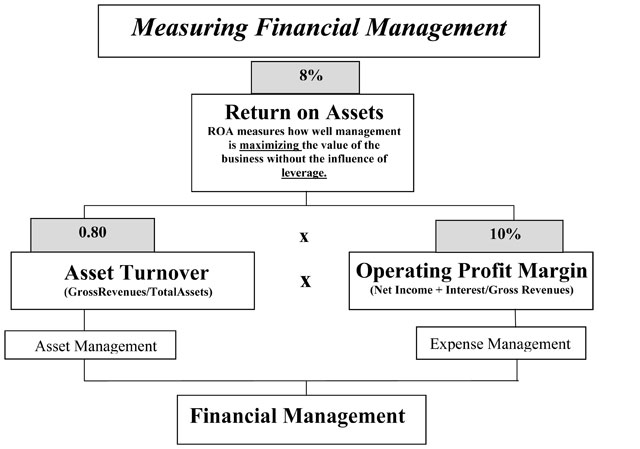
Now that we've rolled all this information into one or two key numbers we have a problem. If the value of ROE is determined to be mediocre, there is no additional information available to diagnose what area or specific problem is causing the less the desirable performance. We can unpack ROA and ROE using a construct called the DuPont equation to develop a means to diagnose and address substandard performance (Figures 1, 2, and 3).
The DuPont equation breaks ROE into three parts, providing a way to audit three key areas of farm management and their contributions to ROE. The three components of ROE evaluate asset management, expense management and debt management. Managing all three of these areas well tends to maximize the value of the business. Comparing the values generated from the DuPont analysis for each of these three areas with industry benchmarks, we can begin to zero in on the areas needing attention. Once these areas have been identified, appropriate subsystem measures can be used to fine tune the identification of the problem.
ROE = Asset Turnover X Net Profit Margin X Leverage
[Asset Management] X [Expense Management] X [Debt Management]
where:
Asset Turnover = Gross sales / Average Total Asset Value
Net Profit Margin = Accrual Net Income / Gross Sales
Leverage = [1/Equity/Total Asset Value]
Let's examine each of the three components of ROE. The first is asset turnover. Asset turnover measures the speed or rate at which the system can produce sales equal to the asset value used to generate them. Asset turnover is industry specific. For lengthy, biological production processes which cannot be speeded up (unlike line speeds on an assembly line), asset turnover is usually low. However, there are several things within management control which affect asset turnover.
The most common limiting factor on farms today is under-employment of existing resources. Assets already purchased and in place are often ineffectively used to generate sales. Asset turnover for a well-run, farrow-to-finish, owned (not contracted) farm will be in the 0.8 to 0.9 range or above. If your values are much lower than this, the subsystem variables to assist you in diagnosing the problem include wean-to-service interval, breeding herd mortality, non-productive sow days, pre-weaning mortality, nursery death loss, average daily gain, pigs weaned per litter, days in the nursery, market weight, parity distribution, farrowing rate, finishing death loss and litters/female/year.
The second component of the DuPont equation is net profit margin. Instead of examining the level of profits we look at accrual net income standardized by (divided by) gross sales. Why standardize profits to gross sales? We can answer with another question. If a business makes a million dollars in profits this year is that good performance? If you're thinking like an economist you answered, "It depends!" If the business made a million dollars profit on five billion in sales we would consider that poor performance indeed. Hence we standardize to sales to examine profit efficiency rather than the level of profits.
The key for most farms here is expense control. Expenses overtime will tend to get out of control. This is almost universal and it applies to household finances as well as farm finances. Good long-term average net profit margins (as defined in the DuPont equation) for owned, farrow-to-finish operations are 6-9%. The key subsystem indicators of expense control are feed expense/unit of gain, feed efficiency, labor expense, interest expense, utilities expense and depreciation expense.
In addition, on the income side, market price, percent lean and average backfat are key subsystem determinants of net profit margin. Comparing the prices you receive for your product with those received by your peers within the industry can be difficult to do accurately. One common misconception among producers is that the same pig should receive the same price at every packer. The price paid is both a reflection of the quality (same for the same pig) and an appraisal of how efficient the packer is at adding value (very different among packers). Just like everyone doesn't bid the same price for available feeder pigs. The price bid is based on quality of the pig and the ability of the finisher to create value.
Other confounders include different products being sold (weaned pigs, feeder pigs, breeding stock, cull animals), different market weights for commercial pigs, different packer buying programs, and the differences in regional markets. An additional difficulty in benchmarking price is the "Lake Woebegone" syndrome (where all the children are above average) in which everyone receives above average prices (premiums) for their products. As the industry moves toward standardized carcass value programs, this price benchmarking will become more meaningful. A common problem in reported prices which thwarts comparison is whether prices are net of transportation, check-off, or yardage.
Feed costs can be evaluated as feed costs per ton, feed costs per pound of gain, or feed costs per pound of lean gain if the required level of detail is available in the record-keeping system. Feed costs per ton can be particularly deceptive. Because of differences in ingredients, ingredient pricing, manufacturing (grind and mix) costs, delivery costs, and measurement or estimation of shrinkage, comparisons of feed costs per ton between farms can be particularly deceptive. Feed costs per pound of gain or per pound of lean gain are much better comparisons; however, benchmarking per-ton feed costs can be useful if the problems with it are understood. The primary ingredients for most swine diets in the U.S. are corn and soybean meal. For diets other than starter diets, these ingredients will make up anywhere from 60 to 90% of the diet. Corn, soybean meal, major minerals, vitamins, trace minerals, and crystalline amino acids will be the ingredients in most diets. Costs of each ingredient, as well as manufacturing and delivery costs, need to be routinely benchmarked to control per-ton feed costs without sacrificing performance.
The components of feed cost per pound of gain are feed costs per ton, feed efficiency, and average daily gain. Feed costs per pound of gain will fluctuate as ingredient costs fluctuate; however, year in and year out, farms with good cost control programs manage to keep feed costs around $0.22 per pound or less. To be at this level, a 250-lb market hog could incur $55 in feed costs. If whole-herd feed efficiency is 3.3 lb of feed per pound of gain, 825 pounds of feed went into bringing the pig to market weight. To stay within the feed budget, feed would have to average $0.067/lb, or $134/ton. Feed cost per pound of lean gain can be evaluated similarly, except that the percent-lean measurement from the packer kill sheet is required. Feed costs per pound of lean gain include the impact of carcass quality as well as feed costs per ton, feed efficiency, and average daily gain. Currently, benchmarking feed costs per pound of lean gain is further complicated by the variety of measurements and measurement devices used for "lean" by the different packers. Standardization of this measurement would allow for more meaningful benchmarking of carcass quality as well as costs per pound of lean gain.
The standardized measure for feed conversion proposed by the NPPC definitions attempts to remove the potential deception mentioned above. The formula is:
(air dry) weight of feed consumed by pigs
live weight gain
The definition is: The total dry weight of feed disappearance divided by live weight gain.
Live weight gain is defined as: Live weight [(salable and transferred) plus inventory change] minus live weight in.
Many established record systems calculate this measure differently. The most common difference is the accounting for total gain versus live weight gain (i.e., either sold out of the building or transferred as a live animal to another building or location, such as a tail-ender building). Those systems which include the gain produced on pigs which are never sold due to death loss will have lower feed conversion values. Systems such as the NPPC guidelines force the full overhead of feed fed to all animals onto the live-weight sold or remaining in further production.
Labor costs are the second largest cost of production on most swine operations. Labor costs per market hog range widely from farm to farm and are difficult to benchmark because of the variety of ways by which labor is accounted. Swine farms with reasonable performance and good cost control spend from $10 to $12 per market hog on labor. These costs can vary considerably by region of the country.
Facility costs (depreciation plus interest) are an important cost of production, especially on new farms. Depreciation plus interest costs may range as high as $16 to $20 per market hog on new state-of-the art farms that are highly leveraged. Utility costs and facility and equipment maintenance vary somewhat by region but also with the age and condition of the facilities. Per head costs of $1 to $4 are not unusual. Veterinary services and medicine are significant costs on some farms, but usually make up no more than 2 to 3% of the cost of production. While costs as high as $10 per head are sometimes observed, a competitive level is $4 or less per head for feed and non-feed medications. Administrative overhead costs vary with the business structure and accounting practices used, but may be a substantial part of total costs of production in some systems.
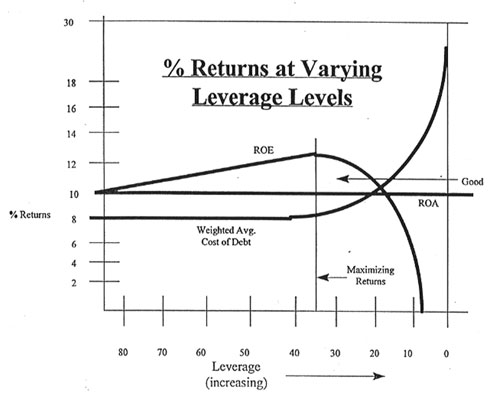
Lastly, managing leverage is critical to maximizing the value of your business. It seems strange to some but the more equity you have, the lower ROE will be for a given level of net income produced. If you are leveraged and profitable, ROE will increase. On the other hand, if you do a poor job of asset and expense management, ROE decreases regardless of your level of leverage.
While we are not recommending opening the flood gates of debt as a means to raise ROE, many profitable producers are under-leveraged. Their profits betray the fact that they are actually destroying their future ability to produce earnings by failure to reinvest in the operation. A cardinal tenet of economics is that scarce resources in a capitalist economy are allocated to their most productive use. If you are a profitable producer of pork, you should consider whether you have chosen a level of debt which is less than optimal. If so, you should weigh the use of additional debt to leverage your business into a larger and more profitable position. If you are an unprofitable producer, the opposite is the case.
Key factors and subsystem efficiency measures used in determining the optimal use of leverage are: working capital, current ratio, working capital/gross revenue, working capital/sow, total equity, term debt/equity, total debt/equity, and the use of leasing and contracting instead of owning assets. Values of the leverage measure above 2.5 must be accompanied by consistent, high profits with price risk protection or the farm can be imperiled by a working capital crisis.
Financial management using a simple construct such as the DuPont equation gives managers the ability to comprehensively assess the long-term production and financial performance of their operation. It rewards those who have taken the time and trouble to keep accurate production and financial records with a source of information to make wise decisions about their future.
In order to illustrate the relationships between asset, expense and leverage management we compare the results of two farms with different ownership structures. The farms are constructed using a detailed simulation process which covers construction, start-up and the first ten years of performance.
Two 600 sow farms are simulated at the 90th and 75th percentile performance for the following variables: litters/mated female/year, born alive, preweaning mortality, weaning age, nursery and finishing mortality, average daily gain in the nursery and finishing phases, and feed efficiency in the nursery and finishing phases.
Percentiles were primarily estimated from the combined PigChamp and PigTales published figures for recent years with additional farm data not covered in these data sets. It would probably be impossible to find a farm where all of these variables were at the same percentile level of efficiency. These were created to establish known benchmark baselines. Table 1 gives the values for each of the variables at the percentiles mentioned.
The farms were simulated under two scenarios. The first was a completely owned, farrow-to-finish operation. The second simulation used identical assumptions except the finishing buildings were contracted instead of owned. In this case, the building costs were reduced by the amount of the finishing complex and space was acquired on a fixed cost per space basis outlined below. The farms were simulated under the two efficiency performances for each asset acquisition strategy.
Additional assumptions include: New construction costs for farrow-to-finish owned = $2,315/sow space. Average grow-finish feed costs = $150/ton. Interest rates for borrowed capital = 10% long-term, 8.5% LOC. Average market price/cwt live for finished animals = $46. Animals were sold at 244 lbs on average.
In the contract finishing simulations, $650,000 in finishing building construction costs were eliminated. The 4,250 spaces were contracted at an annual cost of $144,500 or $34/pig space/year. These assumptions are listed in Table 2. In addition, total farm labor costs were reduced a net 15%, reflecting the labor payment for finishing now paid in the contract payment plus servicing costs. Additional cost reductions were made in utilities, insurance and taxes for the contracting case. It was assumed that net transportation costs would be the same.
Under each simulation, the equity contribution was determined by forcing an initial contribution equal to 40% of year end total asset value for the first year. These figures are given in Table 3, along with the financial outcomes of each scenario.
Note from Table 3 that asset turnover, a measure of asset efficiency, increases between 20% to 30% for the contract finishing scenarios. This is because contractors can achieve the same gross sales with fewer assets on their balance sheet. Note that lower profit farms do not get the same percentage increase in asset turnover because their gross sales are not as high.
Net profit margin in our simulations are lower for the contracting options. This reflects the margin which must be paid above costs (risk premium) to attract contract growers. We have not included any performance change for contract growers compared to owned. Anecdotal evidence gives equal credence to both potential outcomes. You must make a judgment in your unique situation.
Note that in each case, less total equity (and less leverage) is needed for the farms using contract finishing compared to the wholly owned case. Though costs of production per cwt are higher for both the 75th and the 90th percentile contract farms, ROE actually improves for the 90th percentile farm compared to the wholly owned case. This is a very important and crucial lesson. Contract production is not a magic bullet guaranteeing lower costs and more profitability. Normally costs will increase with the use of contract production. However, if compensating gains can be achieved in asset turnover or leverage and those gains can be put to profitable use, contract production can increase ROE and total profitability.
In the case of the 75th percentile producer, compensating gains in asset turnover are insufficient to overcome the increased costs associated with contract production. Assuming the producer had $685,000 in equity to invest, 600 sows could be accomplished wholly owned or ($685,000/$695 equity/sow = 986 sows) 986 sows of farrow-to-finish production could be obtained with contract finishing. The total profit for each scenario would be:
Total Net Income = Net Income/Sow X Total Sow Herd
75th Percentile Wholly Owned: $96,000 = $160/Sow X 600 Sows
75th Percentile Contract Finished: $88,740 = $90/Sow X 986 Sows
In the case of the 90th percentile producer the situation is different. Even though costs of production are higher for each unit, total profitability increases when the same amount of equity is employed by raising sow herd numbers.
90th Percentile Wholly Owned: $189,600 = $316/Sow X 600 Sows
90th Percentile Contract Finished: $266,220 = $270/Sow X 986 Sows
The graph in Figure 4 illustrates the breakeven level of productivity needed to make acquiring assets through contracting more profitable than wholly owned. Keep in mind that this level shifts with a change in any assumption including such things as feed costs, market hog prices, contract rates, levels of performance and so on.
Figure 1.
Figure 2.
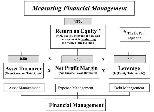
Figure 3.
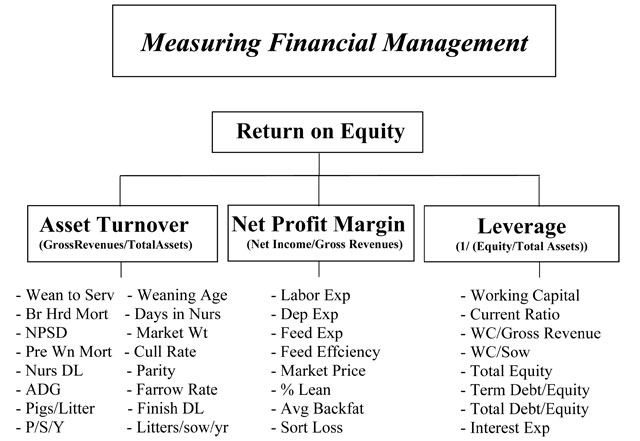
Table 1. Productivity assumptions used in the simulations.
Efficiency Measures |
90th Percentile Value |
75th Percentile Value |
|---|---|---|
Litters/Mated Female/Year |
2.43 |
2.35 |
Born Alive |
11.0 |
10.7 |
Preweaning Mortality |
8.3% |
10.4% |
Weaning Weight |
12 |
12 |
ADG Nursery |
0.87 |
0.79 |
ADG Finishing |
1.65 |
1.57 |
Feed Conversion Nursery |
1.56 |
1.80 |
Feed Conversion GF |
2.85 |
3.00 |
Table 2. Financial assumptions used in the simulations.
Additional Assumptions |
Farrow-to-Finished Owned |
Farrow-Nursery Owned |
|---|---|---|
Cost/Sow Space |
$2,315 |
$1,229 |
Finishing Bldg Cost |
$650,000 |
$144,500 per year |
Long-Term Interest Rate |
10% |
10% |
Line of Credit Rate |
8.5% |
8.5% |
Expected Price/Cwt Live |
$46.00 |
$46.00 |
Marketing Weight |
244 lbs |
244 lbs |
Required Ending 1st Year Equity Percent |
40% |
40% |
Avg GF Feed Cost/Ton |
$150 |
$150 |
Table 3. Results of the simulation for the 90th and 75th percentile farms under each asset acquisition option.
Variables |
75th Percentile |
75th Percentile |
90th Percentile |
90th Percentile |
|---|---|---|---|---|
Asset Turnover |
0.91 |
1.23 |
0.98 |
1.33 |
Net Profit Margin |
7.38% |
4.14% |
13.23% |
11.31% |
Leverage Measure |
1.60 |
1.49 |
1.53 |
1.37 |
Average ROE |
10.71% |
7.59% |
19.92% |
20.59% |
1st Year Equity to Achieve 40% Equity/TA at end of first year |
$685,000 |
$417,000 |
$685,000 |
$417,000 |
Equity/Sow |
$1,142 |
$695 |
$1,142 |
$695 |
Breakeven Cost/CWT |
$40.45 |
$42.08 |
$38.07 |
$39.09 |
Avg Net Inc/Sow |
$160 |
$90 |
$316 |
$270 |
Figure 4.
Index of 1997 Purdue Swine Day Articles
If you have trouble accessing this page because of a disability, please email anscweb@purdue.edu.