Purdue University 2003 Swine Research Report

Analysis of Pig Growth From Birth to Sixty Days of Age

A.P. Schinckel¹, J. Ferrell², M.E. Einstein¹, S.A. Pearce³, and R.D. Boyd^3
1Department of Animal Sciences, Purdue University; ²Primary Nutrition, Dundee, IL; ³PIC USA, Franklin KY

Introduction

The optimization of pork production systems, including the evaluation of alternative management and marketing strategies, requires knowledge of the between and within pig variation in body weight. Little research has been conducted on the growth of pigs from birth to 50 lbs live weight. Heavier pigs at birth and weaning have a competitive advantage and remain heavier throughout their stay in the group. The relationship between the serial live weights and variation in live weight both within and between pigs may be evaluated by the use of nonlinear mixed effects model (Craig and Schinckel, 2001; Schinckel and Craig, 2002). The objectives of this research were (1) to evaluate alternative methods to predict the growth of individual pigs from birth to approximately 60 days of age; (2) to evaluate the relationship of birth weight to subsequent live weights; and (3) to evaluate the relationships amongst the serial live weights.

Materials and Methods

A data set was obtained as part of a swine nutrition research project. Pigs were weighed at birth, weaning (mean age = 19.4 d, SD = 2.4 d), 19 d postweaning (mean age = 38.4 d), and 42 d postweaning (mean age = 61.4 d). The 433 pigs, 220 gilts and 213 barrrows, were assigned to a series of commercially available pelleted diets.

The live weight data were fitted to several alternative growth functions. Two approaches were taken. The first four functions; a modified Bridges, Gompertz, Michaelis-Menten, and exponential equations, were fit to mixed model random effects models using SAS NLMIXED procedures. For these functions, any combination of the fixed parameters could be considered as random and pig-specific deviations predicted. The best single random effects models were evaluated based on the Akaike's Information Criteria (AIC). Then additional random effects were added based on AIC values. The predicted live weight values were calculated for each pig at each age at weighing.

The three functions (modified Bridges, Gompertz, and Michaelis-Menten) were also fit for each individual pig using the NLIN procedure of SAS. Two alternative exponential functions were also fit to the each pig's individual data. The first, a traditional exponential linear quadratic equation, had the form: BW_ij = exp (b_o + b₁ t + b₂ t²) + e_ij where t is age; b₀, b₁, and b₂ are regression coefficients; and e_ij is the random error term. The second has the form: BW_ij = exp (b₀ + b₁ (t + T*) + b₂ (t + T*)²) + e_ij where t is age; T* is a fixed parameter; b₀, b₁, and b₂ are regression coefficients; and e_ij is the random error term. The value for T* was found by fitting the data to a fixed effects model. The values of each variable (b₀, b₁, and b₂) were fit to regression equations from all pigs including the linear, quadratic and cross-product values of the other two variables.

The residual standard deviation (RSD) and coefficient of determination were calculated for each function and method of fitting the BW data (mixed model or fitting data for each individual pig). The mean residual values and the standard deviation of the residual values (RSD) were calculated for each weigh day. The solutions used to fit the nonlinear growth equations had the usual assumption that the residual variance is constant at each measurement age.

The best fitting model was evaluated by comparing the correlations between the serial live weights. With these models, the total variance is the sum of the predicted between pig variance and the within pig variance (RSD²). The predicted correlation between the live weights at two ages was calculated as the covariance between the predicted live weight of the two ages divided by the product of the total standard deviations of live weight at the two ages.

The effect of birth weight on early pig growth was evaluated by two methods. The first method was to regress the predicted live weight at several ages on birth weight. The regression equations included the effect of sex and linear and quadratic effects of birth weight. The second method was to graph the predicted live weight at specific ages on birth weight and to graph the growth of pigs based on five 20-percentile groups for birth weight.

The relationship of the serial live weight was evaluated by two methods. The first method was to regress the actual postweaning BW on weaning weight and any prior postweaning BW. The equations included the linear and quadratic effects of the prior BW. The second method was to regress the predicted postweaning BW's on the predicted prior postweaning weights.

Results

The exponential functions fitted to each pig's data resulted in equations with the lowest RSD values (0.442 and 0.336 kg). Overall, the exponential function of Age + T* provided the best fit (R² = 0.9989) with a value of T* equal to 35.0. However, the RSD's were not equal at the four weigh days, with values of 0.93, 0.99, 0.53, and 0.10 lbs at birth, 19, 38, and 61 days of age. The predicted values from the best exponential functions are very close (-0.10 to 0.06 lb) to the mean actual values of each age (Table 1). The exponential function of age + 35 overpredicted the true variation in birth weight and underpredicted the total variation in weaning weight (Table 1). This exponential function accurately predicted the total variation in the 38 and 61 d live weights.

The b₀ values of the exponential function were found to be a function of b₁ squared, the product of b₁ and b₂ , and b₂ squared (P < 0.0001, R² = 0.72). The b₁ values were found to be a function of b₂, b_0, and b₂ squared (P < 0.0001, R² = 0.96). The b₂ values were found to be a function of b₁ and b₁ squared (P < 0.0001, R² = 0.95). The fact that the values of the three parameters (b₀, b₁, and b₂) have nonlinear relationships with each other makes it difficult to model the true variance-covariance structure of the parameters when an exponential function is fit to each pig's BW data.

The exponential function of age + 35 accurately predicted the individual pig BW at weaning, 19 d postweaning, and 42 d postweaning, with correlations of 0.963, 0.995 and 0.999 respectively. However, the correlation between individual predicted and actual birth weights was substantially lower (R = 0.648). Another indicator of accurate unbiased prediction is the regression of actual on predicted values at each weigh day. The regressions were 0.48, 1.07, 0.96, and 1.00 for birth weight, weaning weight, 19 d postweaning weight, and 42 d postweaning weight, respectively. Based on these statistics, the exponential function accurately predicted the actual BW of the pigs at weaning and postweaning but not from birth to weaning.

The actual and predicted correlations amongst the serial BW's are presented in Table 2. The predicted correlations, which include the residual variance as part of the total variance in BW, should be unbiased predictors of the actual correlations. Overall, the predicted correlations are similar in magnitude to the actual correlations. The actual correlation between birth weight and first postweaning weight (r = 0.531) was greater than the predicted correlation (R = 0.356). The predicted correlation between weaning weight and the first postweaning weight taken 19 d later (R = 0.913) was greater than the actual correlation (R = 0.814).

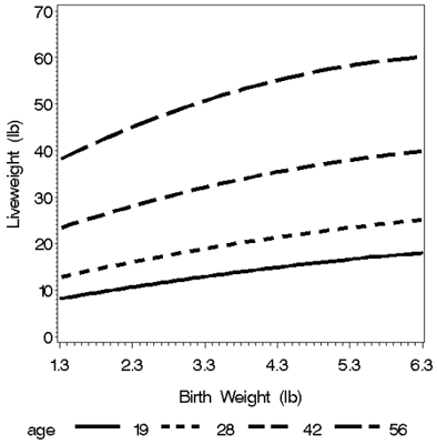
The regression of predicted BW on birth weight is presented in Table 3. Overall, BW at each age had linear-quadratic relationships with birth weight. The relative magnitude and statistical significance of the quadratic effect increased with age (Figure 1). The change in predicted BW at a specific age on birth weight is the derivative of the regression equation and has the form ΔBW/Δ birth weight = b₁ + 2 b₂ birth weight, where b₁ and b₂ are the linear and quadratic regression coefficients, respectively. Because b₂ is negative, the effect of increasing birth weight on subsequent BW decreases as birth weight increases. The effect of increasing birth weight is greater at the lighter birth weights (1.7 to 3.0 lb) than at average (3.72 lb) or above average birth weights. As the pigs increase in age, the effect of increased birth weight increases. At the mean birth weight of 3.72 lb, a 0.1 lb increase in birth weight causes a 0.20 lb increase in BW at 19 d of age and a 0.52 lb increase at 62 d of age.

The live weights taken at 19 and 42 d postweaning had linear-quadratic relationships with prior weights (Table 4). In each case, b₁ was positive and b₂ was negative. At the mean weaning weight of 13.93 lb, a 0.1 lb increase in weaning weight resulted in 0.17 and 0.26 lb increases in liveweight at 19 and 42 d later. Previous trials have found BW's at 28 d postweaning to increase 1.6 to 2.1 lb for each 1 lb increase in 21 d weaning weight. The exponential function fit to each pig reproduced the observed linear-quadratic relationships of the actual BW's.

The pigs were sorted into five 20-percentile groups within sex based on birth weight. The means of the five groups were 2.50, 3.21, 3.63, 4.14, and 5.03 lb and the SD of the five groups were 0.35, 0.13, 0.11, 0.15, and 0.45 lb, respectively. The difference in live weight of the pigs of the five groups increased with age (Figure 2). At the same age, the ADG was similar for pigs of the three average and heavier birth weight groups and lower for two of the lightest birth weight groups (Figure 3). The lightest 20% of the pigs had substantially lower ADG than the other pigs. When ADG was compared at the same weight, pigs of the lowest birth weight had similar ADG to the heavier pigs up to 39 lbs live weight (Figure 4). After 39 lbs body weight, the pigs with the lightest birth weight had lower ADG than the other pigs.

Discussion

The best fit based on RSD values was produced by fitting the exponential function BW_ij = exp (b₀ + b₁ (Age+ T^*) + b₂ (Age + T^*)² ) to each individual pig's live weight data. However, this function still had substantial problems: (1) the function did not accurately predict each pig's birth weight and (2) the RSD's at each weigh day were not equal. These results indicate a lack of fit and the possibility that a more complex function is needed. It is possible that two events limit the pig's maximal growth from birth to 60 d of age. The sow's milk production limits the growth of pigs prior to weaning. Light birth weight pigs tend to nurse the posterior teats, which produce less milk than the anterior teats which are nursed by the heavier pigs. The stress of weaning and sorting also causes a temporary reduction in growth rate. These stressors could cause each pig to deviate from its maximal growth curve, which in turn could cause the residual standard deviations to increase.

Increasing the birth weight of the lightest 20% of the pigs could substantially increase subsequent BW's and potentially reduce variation in BW. Increasing the birth weight of the heaviest pigs will result in only small increases in subsequent BW's. One reason for this curvilinear relationship is the fact that ADG increases rapidly as BW increases. Heavier pigs at the same age are able to grow faster than average pigs, achieve even greater BW at the same age than average pigs, and thus increasingly grow at faster rates. This causes a 0.20 to 0.40 lb advantage in birth weight to become an increasingly greater advantage with time. It is also possible that diets fed on an age basis were not adequate for the lightest pigs, which also tended to have the lowest birth weights. Also, the lightest birth weight pigs may not be able to compete with the other pigs for milk prior to weaning and feed after weaning.

Another alternative is to have a separate production system, including facilities and management, for the lightest pigs at weaning. The nutrition, health program, and facility management could be different for the lightest pigs at weaning. The reduced variation observed in the remaining 80% of the pigs will improve utilization of the larger grow-finish facilities. This reduced variation could result in more precise phase feeding, use of Ractopamine, and marketing at specific target weights.

The modeling of the mean and variance of subsequent BW's is made more complex by the significance of the curvilinear relationships between birth weight and subsequent live weight. Statistical analyses, which assume or only account for linear relationships amongst the serial BW's, would likely not reproduce the actual relationships and variation amongst the serial live weights.

Applications

The growth rate of pigs rapidly increases from birth to 60 days of age. The linear-quadratic relationships between serial body weights makes the modeling of postweaning growth more complex. Increasing the weight of the lightest birth weight pigs could increase the mean and decrease the variance in live weight at subsequent ages.

Table 1. The actual and predicted mean body weights, standard deviation, and correlations of actual and predicted values for each weigh day^a

^a The predicted values are from the equation weighting the two alternative exponential equations which were fitted to the BW data of each individual pig. The total SD is the square root of the total variance, which is the predicted between pig variance plus the residual variance. The correlation (r) is the correlation of the predicted and actual body weights.
^b The pigs were weighed at birth, weaning (mean = 19.4 d, SD = 2.4), 19 d postweaning (mean = 38.4 d) and 42 d postweaning (mean = 61.4 d).

Table 2. Correlations of actual body weights predicted at various ages^a

^a The pigs were weighed at birth, weaning (mean = 19.4 d, SD = 2.4), 19 d postweaning (mean = 38.4 d) and 42 d postweaning (mean=61.4 d).
^b Calculated as the covariance between the predicted values divided by the product of the total standard deviations of the predicted values. Predicted values are the equation BW_ij = exp (b₀ + b₁ (Age + T*) + b₂ (Age + T*)²) + e_ij where T^* = 35.0.

Table 3. Regressions of predicted body weight at various ages on actual birth weight^a

^a The pigs were weighed at birth, weaning (mean = 19.4 d, SD = 2.4), 19 d postweaning (mean = 38.4 d) and 42 d postweaning (mean=61.4 d). Model included effects of treatment, sex, sex by treatment, and the linear (b₁) and quadratic (b₂) effects of birth weight; * P<0 .05, ** P<0.01.
^b The change in BW at the specific age per unit change in birth weight at the mean value of birth weight (3.73 lb).

Table 4. Regressions of actual or predicted body weight on prior actual predicted body weights^a

^a The pigs were weighed at birth, weaning (mean = 19.4 d, SD = 2.4), 19 d postweaning (mean = 38.4 d) and 42 d postweaning (mean = 61.4 d).
^b The change in BW at the subsequent age per unit change in the prior weight at the mean value of the prior age.
*P < 0.10, ** P < 0.01.

Figure 1. Predicted mean body weights for pigs at 19, 28, 42 and 56 d of age relative to birth weight.

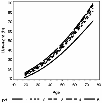
Figure 2. Relationship of body weight to age for five percentile groups of pigs based on birth weight (Group 1 is the lightest 20% and Group 5 the heaviest 20%).

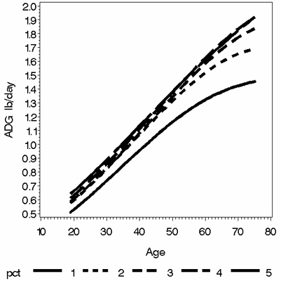
Figure 3. Relationship of ADG to age for five percentile groups of pigs based on birth weight (Group 1 is the lightest 20% and Group 5 the heaviest 20%).

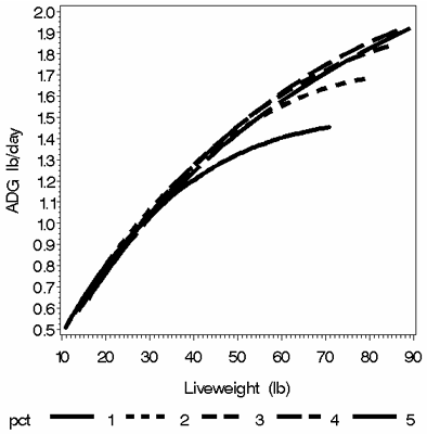
Figure 4. Relationship of ADG to live weight for five percentile groups of pigs based on birth weight (Group 1 is the lightest 20% and Group 5 the heaviest 20%).