Purdue University 1999 Swine Day Report

Contract vs. Independent Pork Production: Does Financing Matter?

M. Boehlje and J. Ray
Department of Agricultural Economics

Introduction

The pork production industry continues to change rapidly. The Midwestern hog production industry, in particular, is experiencing a dramatically changing organizational structure due in part to an increasing cost competitiveness as the industry trends towards larger scales of production, increasingly specialized production, and production utilizing the best advantages technology currently makes available. Many Midwestern pork producers are facing an increasing number and complexity of arrangements to produce pork. This changing structure of production comes at a time when the number of producers involved in pork production continues to decline and the volume of hogs produced grows, reflecting the trend toward fewer but larger production operations.

Numerous Midwestern pork producers are facing the decision of if and how to remain in pork production. The choices available to a producer vary with individual objectives, situational characteristics, and geographic availability of alternatives. While the set of choices for some producers may include facility modernization or enhancement, the investment opportunities analyzed in this study will be limited to those production alternatives requiring a full investment in facilities and equipment. The options we will consider are traditional independent farrow-to-finish production, and different types of contract finishing production. The one dimension common to all possible routes a producer might choose is that they each entail some degree of risk - either the probability of not being able to make debt repayments, or the probability of not achieving an equity return sufficient to compensate the producer for the opportunity cost of investing.

Impact of Debt Financing

The total risk of a project or investment can be viewed as a function of business risk and financial risk. Business risk reflects the risk associated with price and production variability. Financial risk is the probability and magnitude of financial distress that is created by the producer having to meet debt-servicing obligations. A project in which business risk is relatively lower as compared to another may result in the lender being more willing to increase the proportion of debt capital available to the project. For projects with varying degrees of business risk, the difference in the amount loaned between projects reflects an attempt by the lender not to exceed his or her own maximum risk exposure to the project.

Contract arrangements could reduce business risk by stabilizing cash flows, thereby allowing a lender to increase the volume of funds loaned without undue exposure to producer payment default. Thus, the debt provider's risk tolerance threshold impacts how much total capital a producer can access. For example, traditional independent hog expansions can typically expect to access up to 40 to 45% of the capital required as debt funds (Lins, 1997). For a contract arrangement, 80% to even 100% of the capital required may be sourced as debt (Swinton and Martin, 1997; Farmland Industries, Inc., 1996).

The proportion of capital which lenders are willing to provide to invest in pork production facilities is in fact larger for those contract coordinated arrangements in which variability of producer cash flows or business risk is expected to be reduced (Roberts et al., 1998). How this additional debt availability impacts the return on equity might affect which production arrangement a producer will choose to pursue. The impact that changes in the volume of debt funds used have on the equity return of a production arrangement is a critical component of this analysis.

The Analytical Framework

A common approach to analyzing investment options is by using discounted cash flow or net present value analysis. In a typical formulation of this model, the weighted average cost of capital (WACC) becomes the discount factor, because the WACC weighs appropriately the cost of equity capital and the after-tax cost of debt (Fiske, 1986). The WACC is commonly specified as:
           WACC = k_eW_e + k_d(1 - t)W_d
where k_e is the after-tax cost of equity funds (rate of return on equity capital), W_e is the proportion of equity funds used, k_d is the cost of debt funds (interest), t is the marginal tax rate, and W_d is the proportion of debt funds used.

As an alternative to ex-ante specifying the WACC, finding the internal rate of return (IRR) of project cash flows can be viewed as determining the WACC that sets the project net present value (NPV) to zero. If the cost of debt, the applicable tax rate, and the proportion of debt and equity are specified, the rate of return to equity (RRE) becomes the dependent variable in the analysis. Using this approach in a stochastic model, an equity rate of return distribution can be estimated for each project. This equity return distribution can be interpreted as the implicit equity return rate beyond which the project would generate a negative NPV.

If the proportion of debt and equity differ for different investment alternatives as a function of the lender's willingness to finance, the equity return may also differ for these alternatives. More specifically, if a lender is willing to allow those who reduce operating risk under contract production to use more leverage in their business, these producers have the potential to generate a higher equity return with the contract compared to independent production (even if the return on assets is lower) if the cost of debt is less than the cost of equity. Because a distribution of possible equity returns exists, the probability of attaining a specified or desired equity return level adds a critical additional dimension to the analysis. This equity distribution will be evaluated using stochastic dominance and cumulative distribution function techniques (Anderson et al., 1977; Hardaker et al., 1997).

While profitability or the rate of return of a project is an important consideration, the financial feasibility of that project in each period must not be overlooked. Though a project may be profitable, if sufficient cash flows are not generated to cover financial obligations, especially in early project periods, the financial feasibility of the project is put at risk. The probability of meeting all debt obligations in each period using only that period's cash flow is used to assess financial feasibility. To avoid relatively small shortfalls, the cash flow deficit in this analysis must exceed $1,000 before it is classified as financially infeasible.

Model Structure and Data

The analysis technique used is a spreadsheet-based budgeting model that uses @RISK to capture the probabilistic dimensions of pork production. The specific alternative actions the producer will decide among are investing in a 600-head farrow-to-finish operation as an independent producer, or investing in a contract finishing operation consisting of four 960-head buildings under two different contract arrangements. Numerous contract finishing arrangements are available; we will evaluate two that are representative of those commonly found in the Midwest (Farmland Industries, Inc., 1996).

In the independent farrow-to-finish case, the project outlay is estimated at $1,862,037 (Boehlje et. al., 1995). The variability in annual production is modeled using a stochastic death loss term. Stochastic variables are also used for the price received for market hogs and various direct and indirect expenses. Data for these stochastic variables were obtained from Iowa State University record data and market price data for the years 1994 through 1997 (Iowa State University, 1997). Marketing expense, insurance expense, and property tax expense are deterministically set.

Two contracting arrangements are analyzed. The first is a contract finishing arrangement modeled after that offered by a large Midwestern cooperative. The cooperative estimates the facilities and equipment will cost $590,000 for a four-960 head production site. This cost translates into a cost of $153.65 per pig space. The contract arrangement pays a base sum per month per building of $2,600 ($31,200 per building per year) and includes an incentive structure. The original contract term is set at 10 years; at year 10 the contract will be extended for an additional 5 years at a new monthly base payment adjusted for inflation to have the same real value as the original payments. As in most production contracts, the producer is primarily responsible for providing the land, labor, facilities, and management.

The incentive structure has two components. The first component is a tournament ranking system in which a producer could be paid an additional sum based on his or her cost of gain or efficiency ranking as compared against other producers in the same arrangement. The second is a marketing incentive payment tied to the distribution of closeout weights. To model the incentive structures, distributions were developed for each incentive to provide stochastic input into the spreadsheet model.

Table 1 lists the incentive payment based on efficiency ranking per building per closeout. A rectangular distribution from 0% to 100% is used initially to model the tournament ranking and reflects that a producer initially has an equal probability of falling anywhere along the distribution based on his or her relative managerial qualities. As time advances, a producer's ranking is directly tied to the previous period's ranking.

Table 2 illustrates how a producer ranking can change from period to period. If a producer ranks in any of the four middle categories in a prior period, the producer can only advance one ranking, fall one ranking, or stay at the same ranking. If, however, a producer ranks in the top or bottom range, the producer can rise or fall by two ranks. This structure reflects the difficulty of a producer to constantly maintain the top tier incentive due to others trying also to reach that tier. Likewise, this structure reflects a producer's willingness to work so that he or she does not consistently fall in the bottom tier. Discussions with a cooperative representative indicate that producers tend to remain within four of the six rankings over time, but do fluctuate between those four rankings. If a producer falls into the bottom 25% on two consecutive rankings, the payment per building per closeout is reduced by $100 until two subsequent closeouts rank higher. Industry experience with this type of contract suggests that 2.6 closeouts occur per building per year.

The marketing incentive is based on uniformity of market hogs produced. If the producer places at least 60% of a closeout's production between 230 and 270 pounds, he or she will receive an additional $0.50 per pig falling within that window. To estimate the distribution for this payment, mean-variance data which projected the average market hog to have a mean weight of 247 pounds and a standard deviation of 9 pounds (Iowa State University, 1997) was used to seed a simulation consisting of 10,000 iterations to determine how often the condition that 60% of the closeout falls between 230 and 270 pounds is met. This distributional information was then used to calculate the expected marketing incentive per closeout. The marketing incentive was determined to have a mean of $463.40 and a standard deviation of $2.83 for each 960-pig closeout. This mean and standard deviation were then included in the incentive payment structure of each closeout. This result reflects that a producer is often able to qualify for a substantial marketing incentive payment. Discussions with the company representative indicated that for newer contract participants, garnering the marketing incentive tends to occur approximately 90% to 95% of the time, reinforcing the results obtained from the simulation.

The second contract finishing arrangement parallels the previous arrangement with respect to investment and expense characteristics, but uses a different payment and incentive structure. This arrangement is based on a 1,000-head finishing building estimated to cost $140,000. The producer must again provide the land, labor, management, and remaining capital. Direct and indirect expenses are based on the same assumptions used in the first contract finishing arrangement. Instead of a per pig space base payment, a base payment of $11.50 is made for each pig finished. An additional incentive payment of $11.50 is made for each acceptable pig finished which falls below a 2% death loss threshold. Death loss is again stochastic using the same distributional information as for the independent producer. The initial contract term of this arrangement is scheduled to be five years. At the end of year 5 and year 10, the base payment and incentive payment are increased to adjust for inflation so that the payments at those times equate back to the original payment amount. The facility is expected to throughput three turns per year with the contract partner supplying 1,000 acceptable feeder pigs at each turn.

For all three investment options, no project funds will be withdrawn for living expenses, as the labor and management charge is assumed sufficient to cover all living requirements. For simplicity, the terminal value of facilities will be zero at the end of their useful lives, which will be set at fifteen years for each facility type (Boehlje et. al., 1995). Also, investments in net working capital will be assumed to be negligible. No additional capital outlays will be required following the initial capital investment. Direct and indirect expenses inflate at 2.8% annually, and revenues are expected to increase at 2.1% annually (The Wall Street Journal, 1998). The effective income tax rate is set at 28%. The depreciation schedule used is a 10-year, straight-line method. The value of manure as a fertilizer will be assumed to cancel the cost of collection and disposal.

Loan terms for debt financing for all three arrangements are ten years at 10% interest per year. Principal and interest payments will be made once yearly at the end of each year. The producer will pay all labor used including his own at $8.50 per hour. An annual management charge for an independent farrow-to-finish operation is calculated as 3% of gross sales for the year. For the contract finishing options which require much less oversight, 1% of annual gross sales is charged as managerial compensation.

Results

Each investment option was simulated at three levels of debt: 0% debt, 40% debt, and 80% debt. Under the cases with no debt, the calculated equity return (ROE) equals the return to assets (ROA) of the project. While both contract finishing cases analyzed may be 100% financed by the contract partner, 80% debt is the highest level of debt considered to facilitate rate of return comparisons. The following sections will present and discuss the results at each debt level, and then for the independent case leveraged at 40% debt and both the contracting cases at 80% debt.

No Debt

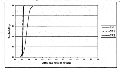
The numerical results for each project with no debt financing are presented in Table 3. Without leverage, the mean calculated equity return (ROE) of the independent farrow-to-finish case at 17.0% exceeds both contract finishing cases at 10.4% and 11.3% respectively. Thus, based on mean returns, the rate of return or profitability of contract production is lower than that of independent production. The graphs of each case's ROE cumulative distribution function (CDF) are found in Figure 1. There is an 80% probability that the equity return will exceed 14.1% for the independent farrow-to-finish case, 9.9% for the efficiency and marketing incentive contract, and 10.9% for the death loss incentive only contract. Invoking first-degree stochastic dominance, the efficient set consists of the independent farrow-to-finish case and contract finishing with death loss incentive only. Second-degree stochastic dominance does not provide any further information in this scenario.

40% Debt

At 40% debt for each arrangement, the mean equity return rises to 23.5% for independent production and 12.5% and 14.0% for the two contracting arrangements respectively, with the same return ordering as in the no debt case (Table 3). The graphs of each project's CDF at 40% debt can be seen in Figure 2. With this leverage position, there is an 80% probability that the equity return will exceed 18.7% for the independent farrow-to-finish case, 11.6% for the efficiency and marketing incentive contract, and 13.3% for the death loss incentive only contract. Again, first and second-degree stochastic dominance lead to an efficient set consisting of the independent farrow-to-finish case and death loss incentive only contract finishing arrangement. While both contracting arrangements are estimated to meet all financial obligations in all periods, the probability of defaulting is .05 for the independent farrow-to-finish investment.

80% Debt

At 80% debt, the equity return for each arrangement approximately doubles as compared to the 40% debt scenario (Table 3). There is an 80% probability that the equity return will exceed 41.8% for the independent farrow-to-finish case, 20.6% for the efficiency and marketing incentive contract, and 25.3% for the death loss incentive only contract with this leverage position (Figure 3). But the probability of each arrangement meeting all period financial obligations drops dramatically for all cases. In fact, the financial feasibility of the efficiency and marketing incentive contract drops below the independent farrow-to-finish case (.33 and .26 probabilities of defaulting, respectively). The probability of defaulting for the death loss incentive only contract increases noticeably to .11.

Differential Leverage

As noted earlier, contract growers can often use more leverage in their operations than independent growers. To analyze this differential impact of leverage on equity returns and financial feasibility, the results for contract growers with 80% debt are compared to independent growers at 40% debt (Table 3). The mean rate of return on equity in this differential leverage scenario is 23.5% for the independent farrow-to-finish case, 23.1% for the efficiency and marketing incentive contract and 27.6% for the death loss incentive only contract.

Graphs of each arrangements respective CDF at these debt levels can be seen in Figure 4. There is an 80% probability that the equity return will exceed 18.9% for the independent farrow-to-finish case, 20.9% for the efficiency and marketing incentive contract, and 25.3% for the death loss efficiency only contract. By first-degree stochastic dominance, the efficient set again consists of the independent farrow-to-finish arrangement and the death loss incentive only contract. At these debt levels, second-degree stochastic dominance establishes that the death loss incentive only contract is the dominating arrangement (results found using stochastic dominance software provided by Dr. Paul Preckel).

With respect to meeting financial obligations, the probabilities of default for independent farrow-to-finish, efficiency and marketing incentive contract, and death loss incentive only contract arrangements are .05, .33 and .11, respectively.

Conclusion

Most discussions of the profitability of contract compared to independent production of pork (or almost any other agricultural enterprise) implicitly or explicitly compare the return on assets (ROA); they ignore differences that might occur in the financing available for these different arrangements which may impact the rate of return on equity (ROE). Studies document that lenders will allow contract producers to use more leverage because the contract is perceived to reduce the business risk of the enterprise, thus allowing it to incur more financial risk. If contract producers can use more leverage, the key issues are what are the implications for the rates of return on equity and the financial feasibility of contract compared to independent production. The analyses presented here provide some insight into these issues in the pork industry.

The results suggest that the different levels of financing available for different types of production arrangements do have a significant effect on the rate of return on equity. The hypothesis that the availability of additional financing in a contract arrangement can enhance a producer's return on equity (ROE) sufficiently to justify entering into a contract arrangement is supported by the analyses presented here. And even without using additional leverage, the results suggest that independent production does not dominate contracts when risk is considered in a stochastic dominance framework.

But in fact the financial risk of some contracts may be underestimated by the lender. The results presented here indicate that at 80% debt, the probability of debt service problems is higher with the efficiency and marketing incentive contract compared to independent production. And with the higher leverage typical with contract production (80% debt) compared to independent production (40% debt), the probabilities of debt service problems are higher with both types of contract production compared to independent production. So although contract finishing in the pork industry may have competitive or higher returns on equity (ROE) compared to independent farrow-to-finish pork production, it may not have as low of financial risk as is commonly thought.

References

Anderson, J.R., J.L. Dillon, and J.B. Hardaker. 1977. Agricultural Decision Analysis. The Iowa State University Press, Ames, IA.

Boehlje, M., et. al. 1995. "Positioning Your Pork Operation for the 21^st Century." Purdue Cooperative Extension Service and Indiana Pork Producers Association.

Fiske, J.R. 1986. "Comparative Analysis of the Return to Equity and Weighted Average Cost of Capital Approaches to Capital Budgeting." Agricultural Finance Review. 46:48-57.

Farmland Industries, Inc. 1996. "Generations III Coordinated Pork Systems." December.

Hardaker, J.B., R.B.M. Huirne, and J.R. Anderson. 1997. Coping with Risk in Agriculture. CAB International, New York, NY.

Iowa State University. 1997. "1997 I.S.U. Swine Business Record." University Extension, Iowa State University.

Lins, David. 1997. "Financing Pork Producers: Challenges and Opportunities." 1997 National Pork Lending Conference. October 7-8, Minneapolis, MN.

Roberts, B., P. Barry, and M. Boehlje. 1998. "Financing Implications for Independent versus Contract Hog Production." Journal of Agricultural Lending.

Swinton, S.M., and L.L. Martin. 1997. "A Contract on Hogs: A Decision Case." Review of Agricultural Economics. 19(1):207-18.

The Wall Street Journal. 1998. Monday, March 30.

Table 1. Tournament incentive structure for contract finishing arrangement.

Table 2. Cost of gain ranking progression.

Table 3. Financial performance of various pork production business arrangements.

Figure 1. Cumulative Distribution Function for Rate of Return on Equity - No Debt.

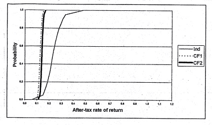
Figure 2. Cumulative Distribution Function for Rate of Return on Equity - 40% Debt.

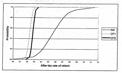
Figure 3. Cumulative Distribution Function for Rate of Return on Equity - 80% Debt.

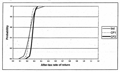
Figure 4. Cumulative Distribution Function for Rate of Return on Equity - 40% Debt for Independent Production, 80% Debt for Contracts.

Index of 1999 Purdue Swine Day Articles

If you have trouble accessing this page because of a disability, please email anscweb@purdue.edu.